Let’s say you send out a survey to 100 random people with a single yes/no question. 80 people response and 60 of those 80 people say yes and the other 20 say no. The classic question in statistics is: what percent of the population would say yes to this question if they all responded? The first approach would be to say 60 of the 80 responded said yes so we would estimate that the population “yes rate” would be 75%. But that assumes that other 20 who didn’t respond would say yes at the same rate as the people who responded. That’s a stretch of an assumption. The question could be “Do you have a cell phone?” and the 20 who didn’t respond don’t have a phone at all.
This leads us to another question: what can we say if we make no assumptions about the people who didn’t respond? We know that 60 of the 100 people did say yes and 20 said no. If we don’t make any assumptions about the other 20 then all we can say is that anywhere between 0 and 20 of them would have said yes if they had responded. So our estimate for the population “yes rate” is anywhere between 60 and 80 percent.
This approach to statistics is called partial identification and was pioneered by econometrics professor Charles Manski. In this post I’m going to formalize some of the mathematics of the situation described above. Then I’m going to fit a model of this situation and get estimates of the lower and upper bounds given sampling error. To do this I’m going to use the probabilistic programming language Stan and call Stan from R.
The math of partial identification
Let’s say \(y\) is a binary variable which represents the answer to the survey question and \(r\) is a binary variable which represents whether someone responds to the question or not. We are interested in estimating \(P(y = 1)\). That is, what is the probability that the answer to the survey question is “yes” for a random person in the population? We can break up \(P(y = 1)\) based on whether they would respond to the survey or not using the law of total probability.
\[P(y=1) = P(y=1|r=1) * P(r=1) + P(y=1|r=0) * P(r=0)\]
To simplify the notation, we can replace of the probabilities with parameters. To summarize them:
\[\begin{align*} \theta &= P(y = 1) \\ \theta_{yr} &= P(y = 1|r=1) \\ \theta_r &= P(r = 1) \\ \theta_{ynr} &= P(y = 1|r = 0) \\ \end{align*}\]
Then we can replace those variables in the equation and use the fact that all we know about \(\theta_{ynr}\) (proportion of nonrespondents who would respond yes) is that \(0 \leq \theta_{ynr} \leq 1\) to get bounds on \(\theta\).
\[\theta = \theta_{yr} * \theta_r + \theta_{ynr} * (1 - \theta_r) \] \[\theta_{yr} * \theta_r \leq \theta \leq \theta_{yr} * \theta_r + (1 - \theta_r)\]
Generative model
Let \(N\) be the number of people we send the survey to, \(r\) be the number of people who respond, and \(y\) be the number of people who say yes. Then we can write a model for how these data were generated based on the unknown parameters above. We will assume a uniform prior for \(\theta_r\) and \(\theta_{yr}\). We will assume that \(y\) and \(r\) are generated by a binomial distribution. And we will specify \(\theta_{lower}\) and \(\theta_{upper}\) based on the inequality above.
\[\begin{align*} \theta_r &\sim Uniform(0, 1) \\ \theta_{yr} &\sim Uniform(0, 1) \\ r|\theta_r &\sim Binomial(N, \theta_r) \\ y|\theta_{yr} &\sim Binomial(r, \theta_{yr}) \\ \theta_{lower} &= \theta_r*\theta_{yr} \\ \theta_{upper} &= \theta_r*\theta_{yr} + (1 - \theta_r) \end{align*}\]
Stan file
The nice thing about Stan is that this mathematical model translates directly to Stan code.
data {
  int<lower=0> N;
  int<lower=0,upper=N> r;
  int<lower=0,upper=r> y;
}

parameters {
  real<lower=0,upper=1> theta_r;
  real<lower=0,upper=1> theta_yr;
}

model {
  r ~ binomial(N, theta_r);
  y ~ binomial(r, theta_yr);
}

generated quantities {
  real<lower=0,upper=1> theta_lower;
  real<lower=0,upper=1> theta_upper;
  theta_lower = theta_r*theta_yr;
  theta_upper = theta_lower + (1 - theta_r);
}
Since we didn’t specify a prior distribution for \(\theta_r\) and \(\theta_{yr}\), Stan automatically chose a uniform distribution.
library(rstan)
library(bayesplot)
library(ggplot2)
library(data.table)
N <- 100
r <- 80
y <- 60
theta_yr_point <- y/r
theta_lower_point <- y/N
theta_upper_point <- y/N + 1 - r/N
survey_data <- list(N = N, r = r, y = y)
fit <- sampling(nonresponse, survey_data)fit## Inference for Stan model: 3af63e94b6c9efbd0049b265a8a1db73.
## 4 chains, each with iter=2000; warmup=1000; thin=1;
## post-warmup draws per chain=1000, total post-warmup draws=4000.
##
## mean se_mean sd 2.5% 25% 50% 75% 97.5% n_eff
## theta_r 0.79 0.00 0.04 0.71 0.77 0.79 0.82 0.87 3085
## theta_yr 0.74 0.00 0.05 0.65 0.71 0.75 0.78 0.83 2777
## theta_lower 0.59 0.00 0.05 0.49 0.56 0.59 0.62 0.68 2768
## theta_upper 0.80 0.00 0.04 0.72 0.77 0.80 0.82 0.87 2820
## lp__ -99.51 0.02 1.00 -102.23 -99.87 -99.21 -98.79 -98.54 1705
## Rhat
## theta_r 1
## theta_yr 1
## theta_lower 1
## theta_upper 1
## lp__ 1
##
## Samples were drawn using NUTS(diag_e) at Fri May 22 14:11:27 2020.
## For each parameter, n_eff is a crude measure of effective sample size,
## and Rhat is the potential scale reduction factor on split chains (at
## convergence, Rhat=1).mcmc_areas(fit, regex_pars = '^theta') + theme(text = element_text(size = 18))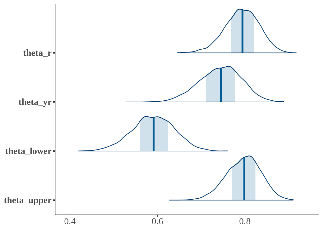
mcmc_scatter(fit, pars = c('theta_lower', 'theta_upper'), alpha = 0.1) + theme(text = element_text(size = 18))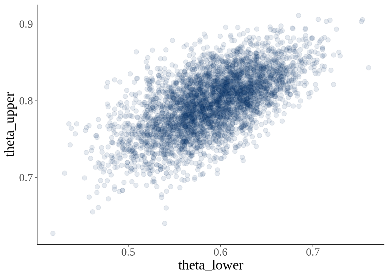
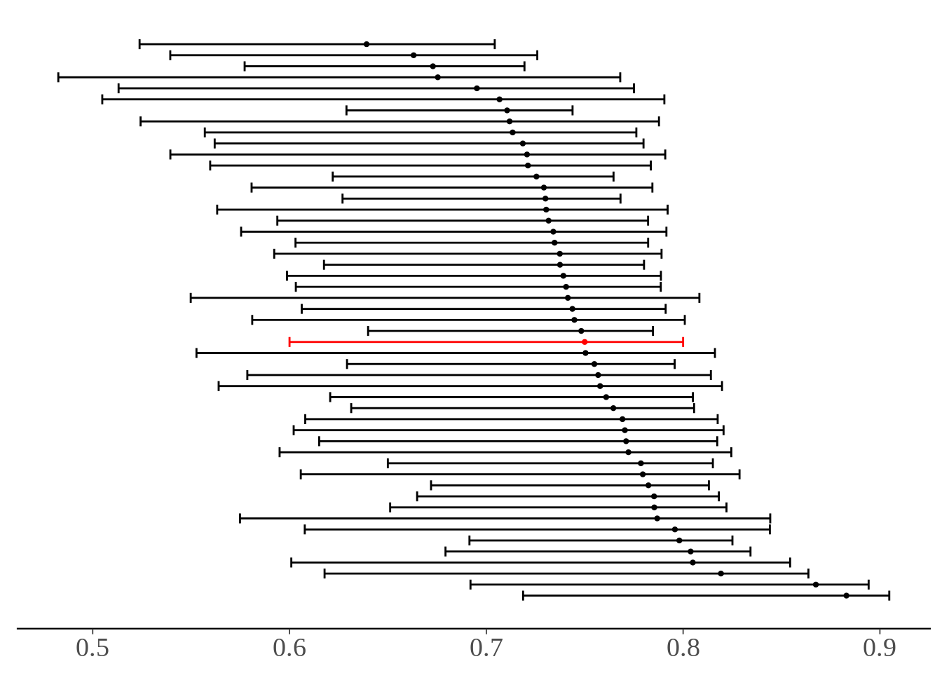
Another way to show our posterior is to plot 50 draws from the posterior of \(\theta_{yr}\) as points and the range of \(\theta\), i.e. \([\theta_{lower}, \theta_{upper}]\), as intervals. Plus, we’ll show our “point estimate” for the interval in red.
num_iter <- 50
DT <- as.data.table(rstan::extract(fit, c('theta_lower', 'theta_upper', 'theta_yr')))
DT <- DT[sample(.N, num_iter)][, point := FALSE]
pointDT <- data.table(
    theta_lower = theta_lower_point,
    theta_upper = theta_upper_point,
    theta_yr = theta_yr_point,
    point = TRUE
)
DT <- rbindlist(list(DT, pointDT))
DT <- DT[order(-theta_yr)]
DT[, iter := 1:.N]

ggplot(DT, aes(xmin = theta_lower, xmax = theta_upper, x = theta_yr, y = iter, color = point)) +
    geom_errorbarh() +
    geom_point(size = 0.8) +
    theme_default() +
    scale_color_manual(values = c('black', 'red')) +
    guides(color = FALSE) +
    theme(
        text = element_text(size = 18),
        axis.line.y = element_blank(),
        axis.ticks.y = element_blank(),
        axis.text.y = element_blank(),
        axis.title.y = element_blank(),
        axis.title.x = element_blank()
    )
)